Building My Robotics Stack, Part 4: From LiDAR to a First Navigation Goal
Part 1 · Part 2 · Part 3 · Part 4
By this point I had a moving robot, a custom wheel-odometry node, and a separate wheel-plus-IMU estimation baseline. The next milestone was to give the robot a view of its environment, build a map, and send a navigation goal.
I approached this as a sequence of interface checks: first a measured obstacle, then a room, then mapping, then navigation. Each layer gave the next one something concrete to depend on.
Before mapping, measure one box
I added a simulated 2D LiDAR and bridged its output to ROS as /scan. Before launching SLAM, I placed a box with known dimensions in front of it.
The box center was 2.0 m away along the forward axis, and its depth was 0.2 m. The expected near face was therefore at 1.9 m, rather than at the center. The ray nearest forward measured 1.907526 m: about 7.5 mm beyond that prediction.
This checked the scanner’s geometry, frame, bridge, and range interpretation together. The scan had 720 rays over approximately a full circle, published at 10 Hz, and used lidar_link with advancing simulation timestamps.
A LaserScan stores ranges by angle index:
angle_of_ray = angle_min + index * angle_increment
After the robot turned approximately +0.504 rad, the box appeared near -0.502 rad in the scanner frame. The sign matters: a stationary world object shifts toward the opposite side of a sensor rotating with the robot.
A room made visibility limits obvious
I then used a bounded room with walls and two obstacles, including a deliberate occlusion case. A planar scan reports the first visible surface along each ray. A nearby box can hide another surface even when the simulator clearly shows that surface exists.
That helped me distinguish a sensor limitation from missing geometry. Moving the robot changes which surfaces are visible; an unseen region is not necessarily empty.
It also made the difference between scan points and a map clearer. A scan is a set of observations from a sensor pose. An occupancy grid combines observations over space and time into estimates of free, occupied, and unknown cells.
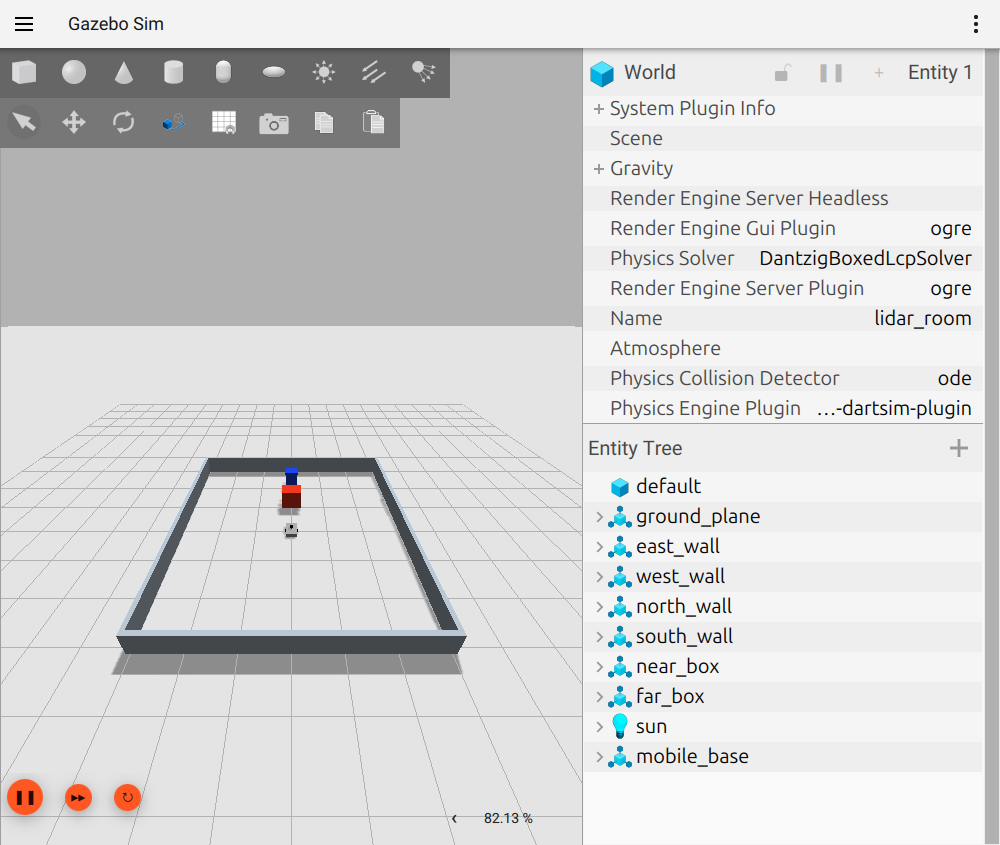
Newly reproduced Gazebo view of the test room. The near red box can hide the farther blue box from the robot’s LiDAR. This capture uses a temporary OGRE rendering override because the default graphics path crashed; it is an illustration of the scene, not a new accuracy experiment.
Building the first occupancy grid
I configured SLAM Toolbox to consume /scan, using the existing robot transforms and simulation time. A dedicated mapping launch composed it with the working simulation/control baseline.
The essential SLAM configuration connects the sensor to the frame chain:
odom_frame: odom
map_frame: map
base_frame: base_link
scan_topic: /scan
mode: mapping
resolution: 0.05
These names have to agree with the transforms and scan messages actually being published. The resolution sets the grid cell size in meters; it does not guarantee map accuracy at that scale.
The frame ownership was central:
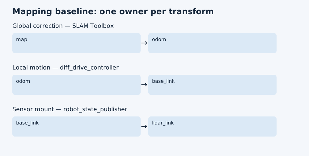
odom supports locally continuous motion. SLAM supplies the correction between that local odometry frame and map as it aligns observations. The robot model supplies the fixed relationship from the base to the LiDAR.
The EKF still had publish_tf: false. Although I had tested its filtered output in the previous phase, this mapping and navigation baseline continued to use controller odometry and its transform. Those are separate integration decisions.
My first room map used 0.05 m per cell and showed a 120-by-120-cell grid. In my notes I recorded sparse free/unknown patterns and an occluded wedge behind the near obstacle. A convincing outline in the raw scan does not mean every grid cell has accumulated enough evidence to be classified.
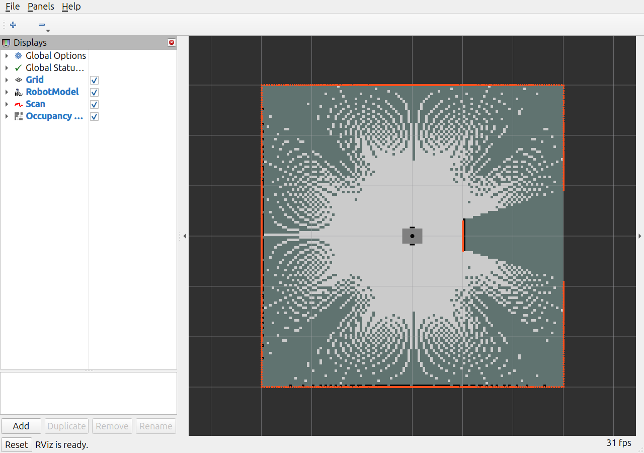
Newly captured from the same temporary visualization run: orange points are scan returns, and the grid contains free and unknown regions. The wedge behind the near box shows the visibility limit from this pose. This is a stationary mapping view, not the historical Nav2 goal run.
I also had to remember that map need not share Gazebo world’s origin. Relative distances and wall spacing are more meaningful first checks than comparing raw absolute coordinates across unaligned frames. I did not record a complete numerical map-accuracy benchmark at this milestone.
A map is one input to navigation
Nav2 needed more than /map: a continuous local odometry transform, robot footprint, obstacle observations, compatible velocity commands, and active lifecycle nodes.
The global costmap uses map; the local rolling costmap uses odom. Both observe /scan. I configured a rectangular footprint based on the robot’s 0.40 by 0.37 m extent, with additional costmap padding.
The command interface also needed attention. This robot’s controller consumes TwistStamped. I configured stamped velocity messages throughout the navigation command chain:
Nav2 controller / behaviors
    -> cmd_vel_nav
    -> velocity_smoother
    -> cmd_vel_smoothed
    -> collision_monitor
    -> /diff_drive_controller/cmd_vel
Checking the final topic showed one publisher from the collision monitor and one controller subscriber. That verified the intended wiring through the safety stage. It does not by itself establish comprehensive obstacle-avoidance or safety performance.
A dedicated launch file and project-owned configuration made this command path repeatable.
A short goal exposed a configuration mismatch
The first short-goal test caused recovery behavior near the destination. The command chain worked, but several tolerances disagreed.
The planner could accept an endpoint up to 0.25 m from the request, while the goal checker required 0.15 m. The progress checker demanded 0.20 m of movement, which was too coarse for this short, slow approach.
The final configuration reduced planner tolerance to 0.05 m and required 0.02 m of progress within 15 seconds. With those settings aligned, the same short goal completed normally.
This was a useful integration lesson: components can each be functioning while their acceptance conditions make the combined behavior fail.
What “goal succeeded” meant here
The requested goal was (0.5, 0.0) in map. Nav2 reported SUCCEEDED with error code zero. The final controller odometry was approximately (0.3504, 0.0003) m, and the map-to-base transform independently showed approximately the same location.
Stopping roughly 0.15 m before the requested point was consistent with the configured goal tolerance. It would be misleading to call that exact arrival at 0.5 m.
I recorded the lifecycle states, costmap publication, final command-topic connections, and action result alongside the final pose so that success meant more than seeing the robot move.
This milestone demonstrates a repeatable mapping-and-navigation bringup and one successful short goal in the known test room. It does not yet establish autonomous exploration or performance across diverse environments.
Looking back across these four stages, the strongest progress has been learning to connect models, measurements, frames, and acceptance criteria. The larger multi-robot goal remains ahead, but I now have a single-robot baseline whose behavior I can trace and test.