Building My Robotics Stack, Part 1: From a Robot Model to Controlled Motion
Part 1 · Part 2 · Part 3 · Part 4
I’ve recently started working on this personal project, alongside my other robotics work. Different from what I do in research and the robotics club (where lots of existing tech is used to speed up development), I’m building this from scratch, and without much AI coding. So part of the goal is to get this full-stack robotics experience by myself.
My long-term goal for this project is a group of robots that can explore and map together. Before coordinating several robots, I wanted to understand one: how its model becomes a moving body, how a velocity command reaches its wheels, and how I can tell whether the system is working.
This is the first entry in that build log. By August 11, I had a differential-drive robot running in Gazebo through ros2_control, with wheel state feedback and controller odometry. Getting there meant separating several things that initially looked like one task: describing a robot, displaying it, simulating it, and controlling it.
A model that looks right still needs physics
I started with a URDF description expanded through Xacro. URDF describes links and the joints connecting them; Xacro lets me express repeated structure and dimensions without copying every value by hand. For this base, the important moving joints are the two continuous wheel joints.
The model has three descriptions of each physical link:
- Visual geometry: what I see.
- Collision geometry: what the physics engine uses for contact.
- Inertial properties: mass, center of mass, and resistance to angular acceleration.
These descriptions need to tell a consistent story. A wheel can look perfectly placed while its collision shape touches the ground somewhere else. A body can render correctly while having an implausible inertia. Those discrepancies matter once gravity, contact, and acceleration enter the picture.
RViz was useful for inspecting the structure and frames. Gazebo was the next test because it adds physical behavior. I checked the model before adding a more complicated control architecture: could it spawn, sit on the ground, and behave plausibly?
That ordering made debugging more manageable. If spawning failed, I could investigate model loading and geometry without also wondering whether a controller had activated.
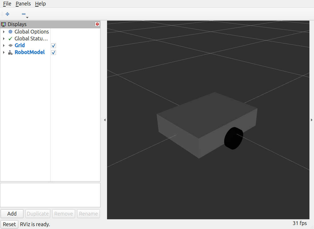
Newly captured RViz view of the August 11 model, reconstructed from its saved revision. Joint-state publication supplies wheel transforms; this view demonstrates the model, not physical driving.
Spinning a wheel in RViz is a different milestone
One distinction I wrote down was the relationship between joint states and movement.
joint_state_publisher can supply joint positions so that robot_state_publisher can compute transforms from the model. Moving a wheel joint in that setup changes how RViz displays the wheel. It does not apply a torque, simulate ground contact, or propel the base.
Once I moved to ros2_control, joint_state_broadcaster supplied joint states from the simulation interfaces instead. robot_state_publisher still used those states to compute link transforms.
The similar names hide different jobs. Understanding those jobs helped me ask better debugging questions: am I looking at a display of a joint angle, a measured simulated joint state, or an actual command to an actuator interface?
First motion: use a small baseline
For the first drive test, I used Gazebo’s DiffDrive system plugin. It takes a body velocity command and drives the simulated wheel joints. The plugin needed the wheel names, wheel radius, and wheel separation.
For this robot, the wheel radius is 0.05 m, and the wheel centers are 0.34 m apart. Those dimensions later become kinematic parameters, so they need to agree across the model and controller configuration.
I first established that the robot could move in Gazebo, then connected ROS commands through ros_gz_bridge. A topic named /cmd_vel in ROS and a topic with the same name in Gazebo Transport are still on separate communication graphs. The bridge translates between them; the drive plugin performs the control-related work.
This gave me a simple working reference before introducing controller management and hardware interfaces.
Moving to ros2_control
The next step was a separate simulation path using ros2_control. The learning value was understanding the boundary between controller behavior and the mechanism that applies commands to joints.
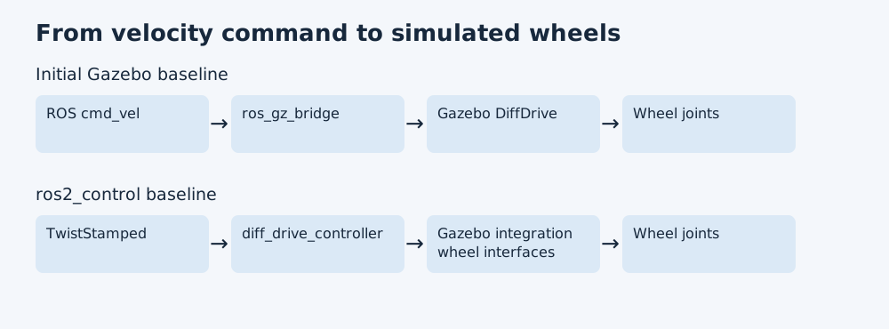
These are alternative bringup paths. The two drive systems should not command the same wheels together.
In the new path, diff_drive_controller accepts a body velocity command, converts it to left and right wheel velocities, and writes those commands to wheel velocity interfaces. Gazebo’s ros2_control integration connects those interfaces to the simulated joints. Joint position and velocity state come back through the corresponding state interfaces.
The controller configuration makes the geometry explicit:
diff_drive_controller:
  ros__parameters:
    left_wheel_names: ["left_wheel_joint"]
    right_wheel_names: ["right_wheel_joint"]
    wheel_separation: 0.34
    wheel_radius: 0.05
    base_frame_id: base_link
    odom_frame_id: odom
This is an excerpt, rather than a complete controller configuration. The migration brought together the model interfaces, controller configuration, and launch changes.
I kept the initial Gazebo path available while validating the new one. That meant I had a known working comparison instead of replacing every moving part at once.
Following a command all the way through
The controller path uses /diff_drive_controller/cmd_vel with a TwistStamped message. That detail matters: matching a topic name is insufficient if the producer and consumer disagree on its message type.
I checked active controllers and available interfaces, commanded a small forward motion and turn, and inspected /joint_states, /diff_drive_controller/odom, and TF. Each observation answers a different question:
- Active controllers show that the control components loaded and activated.
- Wheel states show that the simulated joints respond.
- Odometry describes estimated base motion from wheel feedback.
- TF makes the relationships between frames available to other components.
The repeatable launch file brought these responsibilities together so I could start subsequent experiments from the same baseline. Launch files became part of how I described the system, rather than just a way to avoid typing commands.
What this milestone gave me
I now had a robot whose command and feedback paths I could explain. I also had a clearer boundary between using existing robotics software and understanding what it does. I configured the standard differential-drive controller; I had not written a motor controller or demonstrated behavior on physical hardware.
That working simulation was the foundation for the next question: could I take the wheel states myself and recover the robot’s motion?