Building My Robotics Stack, Part 3: What to Trust in Sensor Fusion
Part 1 · Part 2 · Part 3 · Part 4
After implementing wheel odometry, I added an Extended Kalman Filter using robot_localization. My goal was to learn how measurement selection, frames, timestamps, and uncertainty affect an estimate—not simply to produce a smoother-looking topic.
The most useful outcome was a result I could not honestly describe as “adding an IMU improved accuracy.” The filter worked, but the experiments taught me something more specific about when to trust its inputs.
Start with a measurement contract
An EKF alternates between predicting a state and correcting that prediction with measurements. The corrections depend on the uncertainty assigned to the prediction and the measurements. A sensor value without a meaningful frame, time, or uncertainty is an incomplete input.
I began with the custom /student/odom topic and enabled only forward velocity and yaw rate. I left the wheel-derived position and heading disabled because they were accumulated from the same wheel data. Feeding more fields from one source does not automatically provide more independent information.
I also kept the problem planar with two_d_mode: true and disabled EKF TF publication. The controller already owned odom -> base_link; introducing a competing transform publisher would make the experiment harder to interpret.
The input mask makes that choice explicit. Here is the relevant configuration excerpt; each group follows the state order shown in the comments:
two_d_mode: true
publish_tf: false
odom0: /student/odom
odom0_config: [false, false, false,  # x, y, z
               false, false, false, # roll, pitch, yaw
               true,  false, false, # vx, vy, vz
               false, false, true,  # roll/pitch/yaw rates
               false, false, false] # ax, ay, az
imu0: /data/imu
imu0_config: [false, false, false,
              false, false, false,
              false, false, false,
              false, false, true,
              false, false, false]
Only the selected variables influence the filter as measurements from those sources. Disabling wheel pose does not mean the filter stops estimating pose; it predicts and updates its state using the selected velocity measurements.
This was configuration and integration of an existing filter implementation. My custom component was the wheel-odometry node, not the EKF algorithm itself.
Covariance expresses confidence
In my odometry notes, I separated what the wheel model observes reasonably well from what it cannot directly measure. Forward motion gets moderate confidence. Lateral slip and unobserved 3D motion should not appear as certain merely because their message fields contain zeros.
Covariance entries are variances, not standard deviations. A larger measurement variance generally reduces that measurement’s influence in a correction. The actual filter response also depends on process uncertainty, other measurements, and update history.
For the first IMU integration, I selected only angular_velocity.z. The sensor had a fixed imu_link, simulation timestamps, and a roughly 50 Hz stream. I checked the raw interface before adding it to the filter.
The existing wheel yaw-rate variance was 0.1 (rad/s)^2; the simulated gyro reported approximately 4e-8 (rad/s)^2. That enormous difference in stated confidence gave the gyro a strong nominal influence when the sources disagreed.
Compare filters using the same recording
Rather than drive two separate trajectories, the experiment recorded raw wheel odometry, IMU data, simulation clock, and Gazebo model pose once. The same inputs were replayed through a wheel-only EKF and a wheel-plus-IMU EKF.
Both filters fused wheel forward velocity and yaw rate. The second additionally fused IMU yaw rate. Both published at approximately 30 Hz.
The motion sequence included positive, negative, and faster positive rotations followed by a stop. Comparing against Gazebo heading provided a reference beyond the command: commanding a particular turn rate does not prove the body actually followed it.
There was an important measurement limitation. The pose bridge lost source names and timestamps, so the analysis identified the robot transform and aligned receipt times through the recorded simulation clock. Small heading differences can therefore include timing and interpolation effects.
Stable fusion did not mean consistently better heading
The baseline filters had the correct turn signs and remained stable. The fused filter followed the gyro closely, as expected from the relative variances. It did not consistently improve heading accuracy in this ideal, low-slip simulation.
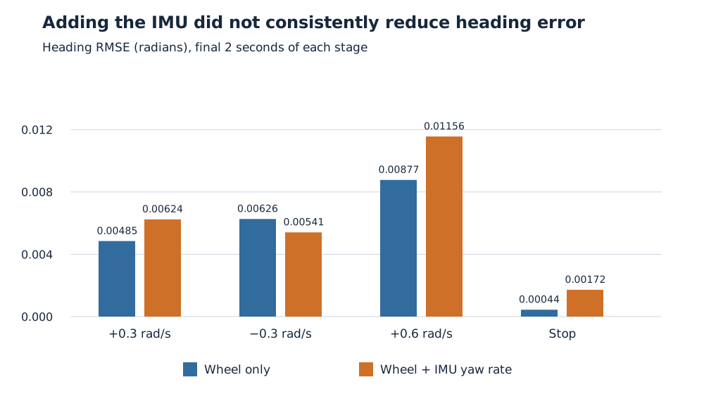
Values are heading RMSE against Gazebo heading during the final two seconds of each stage, not whole-run error.
For example, the fused heading RMSE was 0.00624 rad during the positive slow turn, compared with 0.00485 rad for wheel-only. In the negative turn, the fused result was slightly better. The differences were small, and the reference alignment had limitations.
The supported conclusion was that the two-source integration worked. This experiment did not demonstrate a general accuracy advantage from adding an IMU.
Make the sensors disagree on purpose
The next test altered the recorded IMU yaw rates with a fixed +0.03 rad/s bias and Gaussian noise with 0.05 rad/s standard deviation. Two filters received the same altered samples, wheel data, and trajectory, while using different declared IMU variances.
One retained the tiny native variance. The other used 1.0 (rad/s)^2 as a deliberately conservative sensitivity setting. At the stop stage, heading RMSE was approximately 1.159 rad for the understated-variance case and 0.106 rad for the conservative case.
That demonstrated how strongly an overconfident measurement can pull the estimate. It did not make 1.0 a calibrated sensor variance. Increasing uncertainty can suppress a biased input; it does not estimate or remove the bias.
I kept the baseline and controlled-disagreement results separate: the first tests integration on native measurements, while the second tests how declared confidence changes the response to deliberately altered measurements.
Noise and bias need different questions
A separate stationary window contained 950 samples over 19 seconds. The native gyro variance was 3.822e-8 (rad/s)^2, close to its reported 4e-8. Its small mean did not establish a nonzero bias within the sampling uncertainty of that window.
That supported retaining the native yaw-rate covariance and applying no bias correction for the current baseline. It did not establish long-term bias stability across starts or warm-up conditions.
The deliberately biased stream illustrated the other side: replacing its variance with the measured random-noise variance still left substantial heading error. Honest random-noise variance does not account for a fixed offset in the mean.
Why I left orientation fusion disabled
The IMU also supplied an orientation quaternion, but every saved orientation covariance entry was zero. For an IMU message, all-zero covariance means unknown uncertainty—not perfect certainty.
A rotated-spawn check clarified the reference: with the robot at approximately 1 rad world yaw, the IMU yaw started near zero. After a turn, the same offset remained. In this setup, the reported yaw was relative to startup orientation.
That is a usable observation only after defining the intended reference and an appropriate uncertainty model. I therefore kept orientation fusion disabled rather than adding another field just because it existed.
What I gained from this phase was a more disciplined way to discuss localization: specify what each source measures, compare on shared evidence, and keep conclusions within what the experiment actually tested.